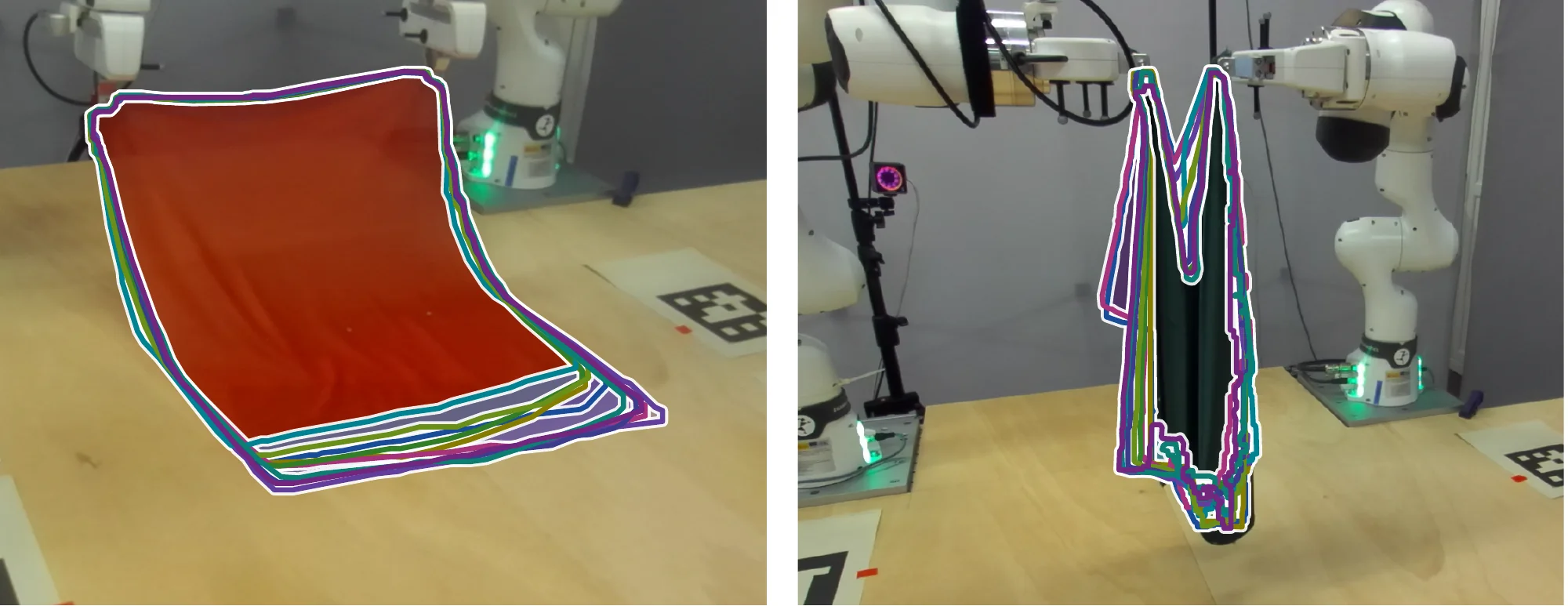
Terminal cloth outlines of ten identical rollouts on one frame, for the swing place (right) and the inward gripper motion (left).
4dynamic tasks
3fabrics
27configurations
269rollouts
19markers at 100 Hz
30 Hzstereo video
1 kHzrobot logs
4simulator twins
Abstract
Although cloth is known to exhibit different outcomes under repeated fast dynamic motions, even when the same trajectory is applied, this variability has not yet been systematically characterized. Quantifying it is essential to assess the reliability of learned manipulation policies and the extent to which simulation can reproduce real-world behavior. To study this, we execute the same trajectory ten times across four dynamic tasks, two of which are novel, each tested with three cloths of very different properties and at up to three execution speeds, with a total of 269 recorded rollouts. For all of them, we record small marker positions on the cloth and synchronized stereo camera. We then formalize different metrics to quantify variability, and our results show how it is significant in every test condition, in most cases one to three orders of magnitude above the repeatability inherent to the robot and sensing noise. Our results also show variability is driven mainly by the cloth physical properties but also grows with speed. By replaying all the rollouts in four calibrated modern cloth simulators, we show that none of them can reproduce the variability magnitude we observed in real cloth, nor its ordering. Together with our analysis, we publish the dataset with synchronized OptiTrack, vision and robot logs and their corresponding simulator twins.
Video
Three minutes, narrated, with captions: the phenomenon, the recording cell, the four tasks, the variability metric, the camera-only analysis and the simulator replays. The ICRA attachment as submitted.
Setup and tasks
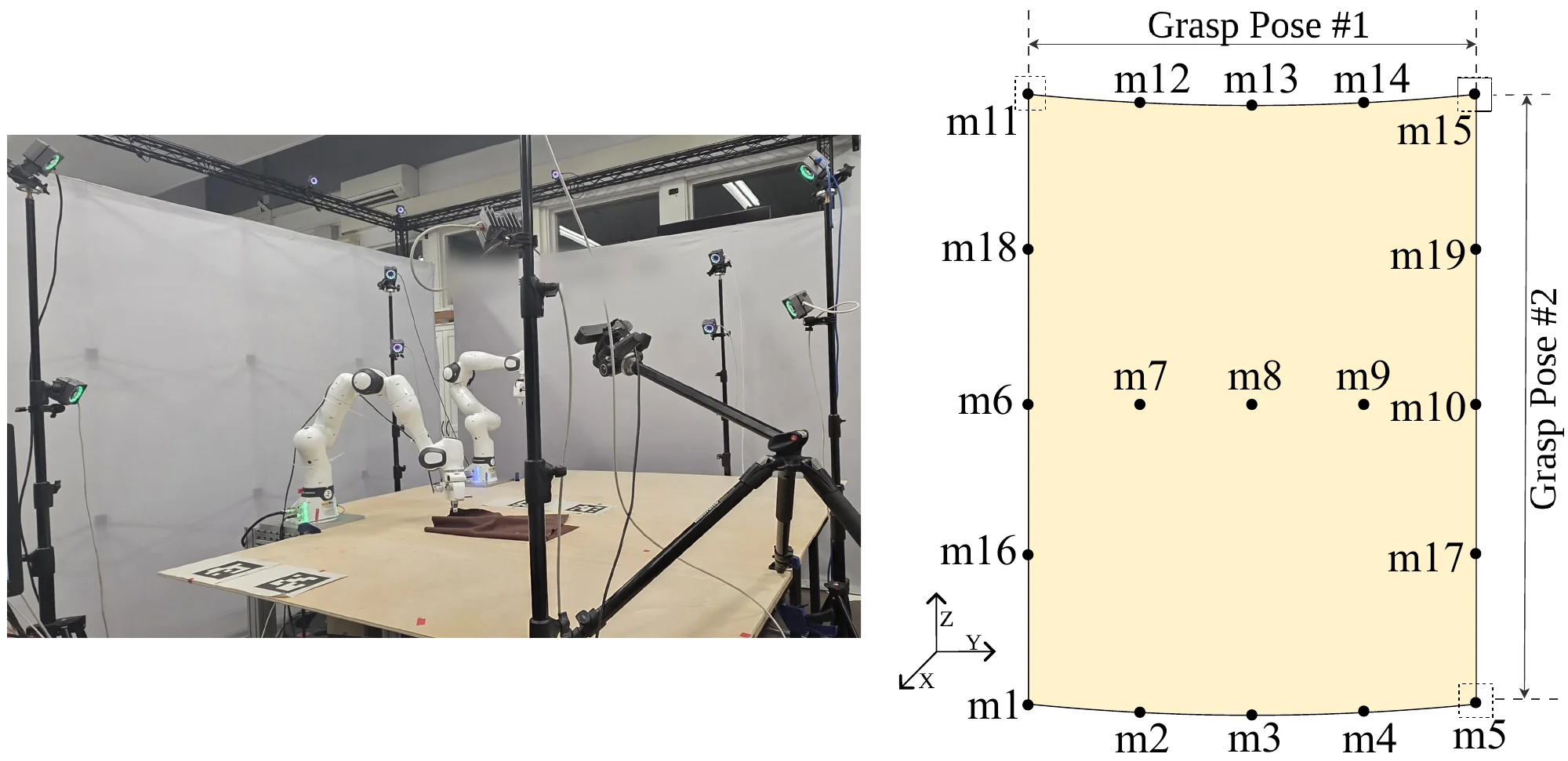
Two Franka Research 3 arms with default Franka Hands stand side by side across a table. Each rollout replays one recorded trajectory in open loop. The trajectories of tasks 1, 2 and 4 come from a teleoperated demonstration, while a linear scripted trajectory planned in joint space is used for task 3. Speed is varied by a time scale ts relative to the recorded speed (ts < 1 is faster). The cloths measure 0.70 × 0.50 m and carry 19 retroreflective markers; an OptiTrack system tracks them at 100 Hz and a ZED 2i stereo camera records the scene at 30 Hz.
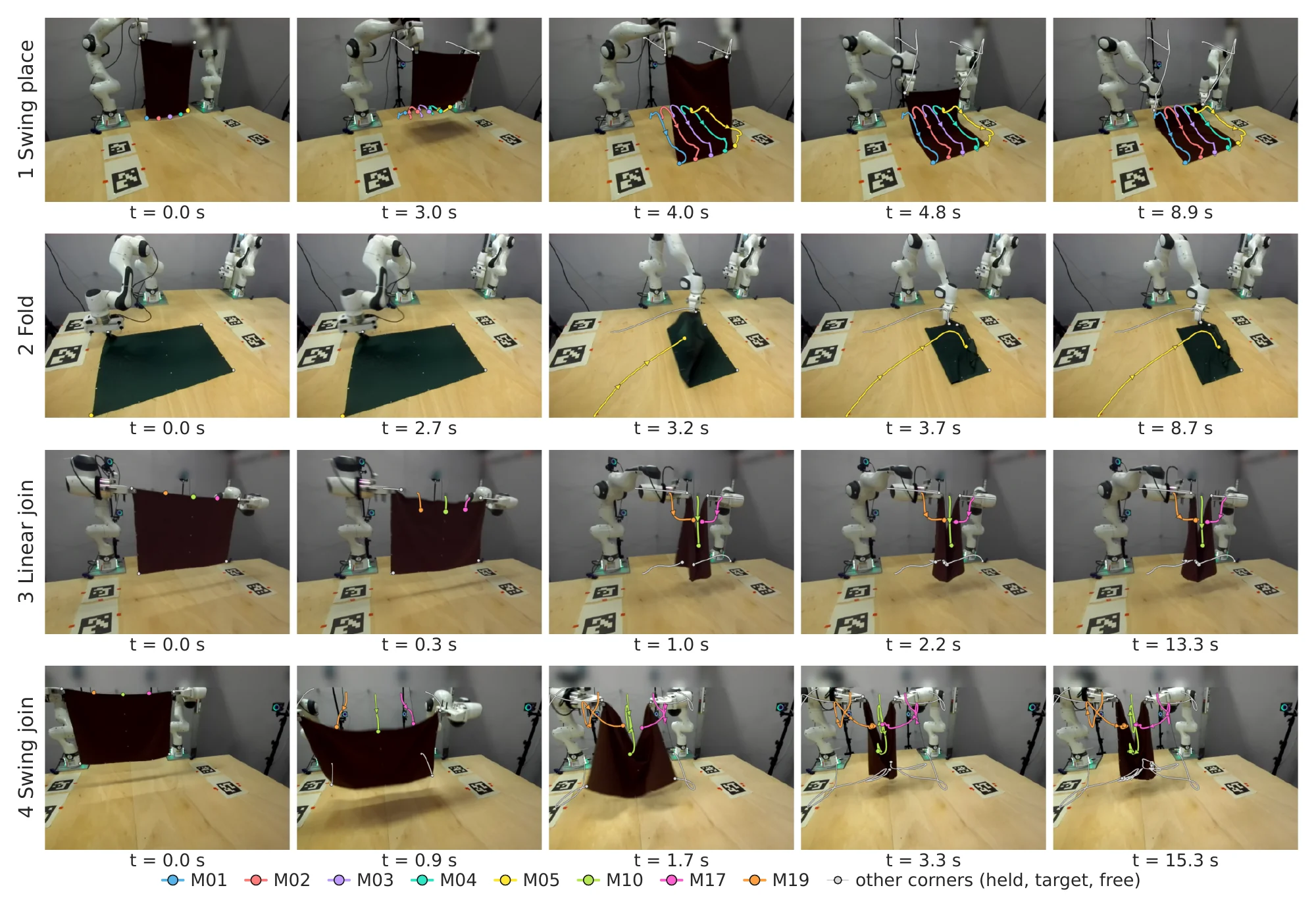
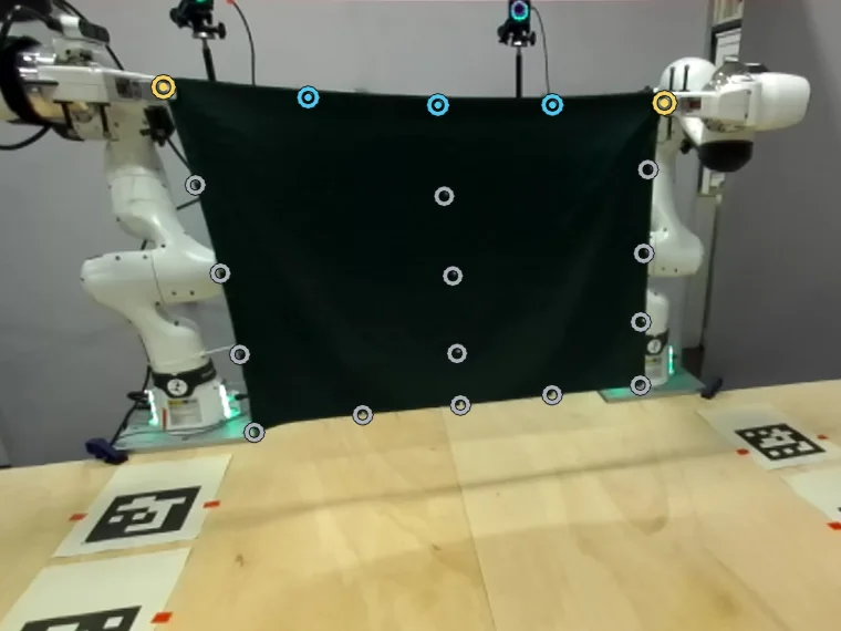
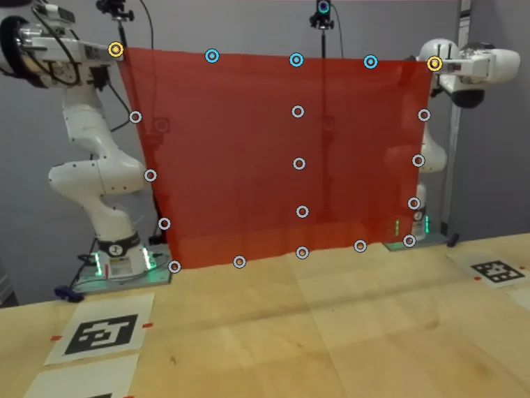
The bimanual cell with the OptiTrack cameras (left) and the 19-marker layout on the cloth (right). Five frames of one rollout per task. The markers whose variability is studied are colored and tracked in the camera view; other relevant markers are gray.
1 · Swing place
Both arms hold the short edge M11–M15, swing the cloth forward and lay it flat without releasing it.
D̄ is evaluated on the resting position of the free edge M01–M05 on the table, and the floor ε on the grasped corners M11 and M15.
2 · Fold
The right arm holds the corner M01 and folds it towards M11; the edge M11–M15 stays on the table and the free corner M05 is aimed at the corner M15.
D̄ is evaluated on the resting position of M05 on the table, and the floor ε on the held corner M01.
3 · Linear joinnovel
The grippers hold the corners M05 and M15 and move toward each other along a straight line, stopping before contact; the cloth ends hanging crumpled in the air.
D̄ is evaluated in 3-D on the top-edge markers M17, M10 and M19, together with the side to which the cloth buckles, and the floor ε on the grasped corners M05 and M15.
4 · Swing joinnovel
Same goal as the linear join, with a swing before the inward motion, meant to control the buckling side.
The same measurements as in task 3.
Configurations
#
Task
Object
Time scale ts
Regrasp
1
Swing place
1 cloth (b)
0.8, 1, 1.2
No
2 cloths (g, r)
0.65, 1, 1.35
No
2
Fold
3 cloths
1, 1.4
No
3
Linear join
3 cloths
1
No
1 cloth (g)
1
Yes
4
Swing join
3 cloths
1, 1.5
No
2 cloths (g, r)
1
Yes
b, g and r stand for the brown, green and red cloths. Ten rollouts per configuration, nine in one (swing join, brown wool, ts 1.5).
Speeds side by side
In the video three configurations of the swing place run on one clock, then the swing join and the fold. Here, for each task, one rollout of every configuration plays from the moment the robot starts to move, one row per cloth and one tile per speed, with the regrasp configurations tagged. At real speed the fast execution lands first.
D̄ per configuration · brown wool 8 / 9 / 5 mm · green satin 47 / 28 / 23 mm · red chiffon 81 / 39 / 33 mm
Captions of this scene in the video (swing place)
The same command at three speeds, started together
The swing join on the green satin at its two speeds and with a regrasp before each replay · the fold on the red chiffon at its two speeds
Fabrics
The cloths have the same size but very different physical properties. The brown cloth is a thick wool fabric with high stiffness and low elasticity. The green satin is much lighter with less stiffness and friction but a similar elasticity. The red is a very light chiffon fabric that is very elastic, very soft, and has the lowest friction coefficient.
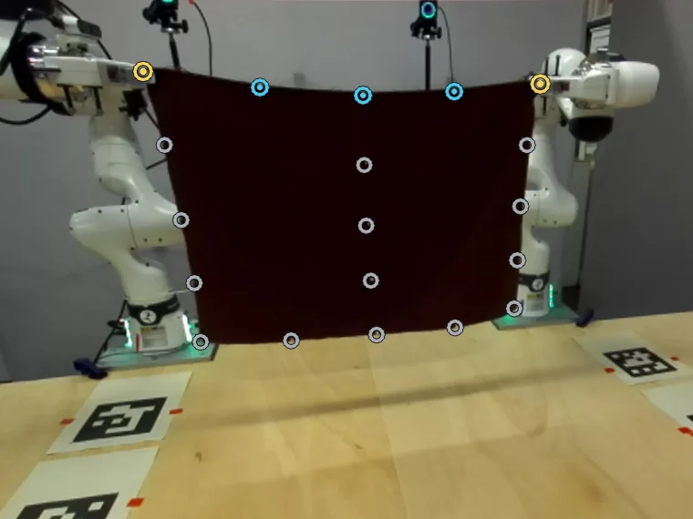
The three cloths at the start of a swing join, held by the long edge at M05 and M15. Markers by role: grasped corners M05, M15 · free edge M17, M10, M19 (D̄) · other markers.
Each axis runs from zero to the largest value among the three cloths. Elasticity is the largest of its three directions.
brown wool
green satin
red chiffon
mass (g)
139
35
27
areal density (g/m²)
400
100
76
friction coefficient μ
0.68
0.48
0.40
elasticity† (%)
8 / 1 / 17
1 / 12 / 18
20 / 38 / 13
drape stiffness (%)
9.5
5.9
3.1
† Elasticity along the short, long and diagonal edges, respectively.
Results and analysis
Comparison of variability across tasks
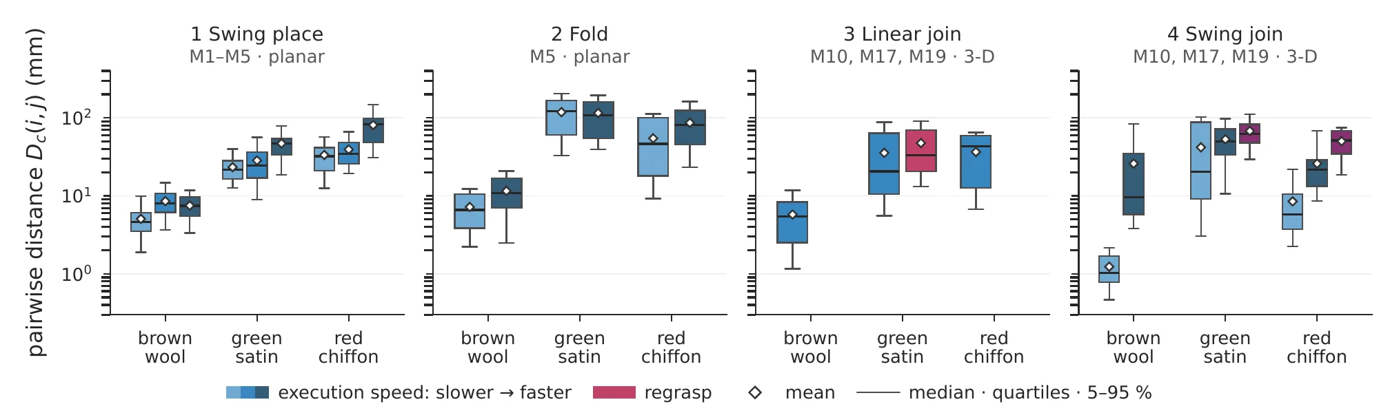
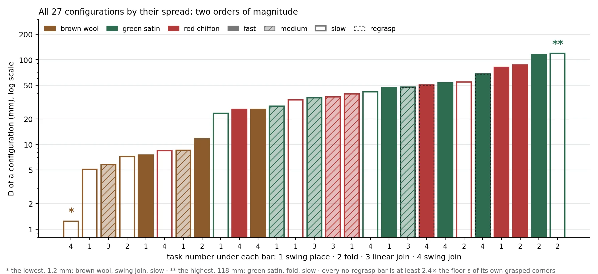
The whisker boxes in the figure show the pair distances of the 27 configurations and their means D̄c. The y-axis is logarithmic because D̄c spans from 1.2 mm, for the brown cloth in the slow swing join, up to 118 mm for the folding with the green satin, a factor of 96. Every no-regrasp configuration exceeds the floor variability of its grasped markers by at least 2.4×, and most by one to three orders of magnitude, so in all cases it is a non-negligible phenomenon.
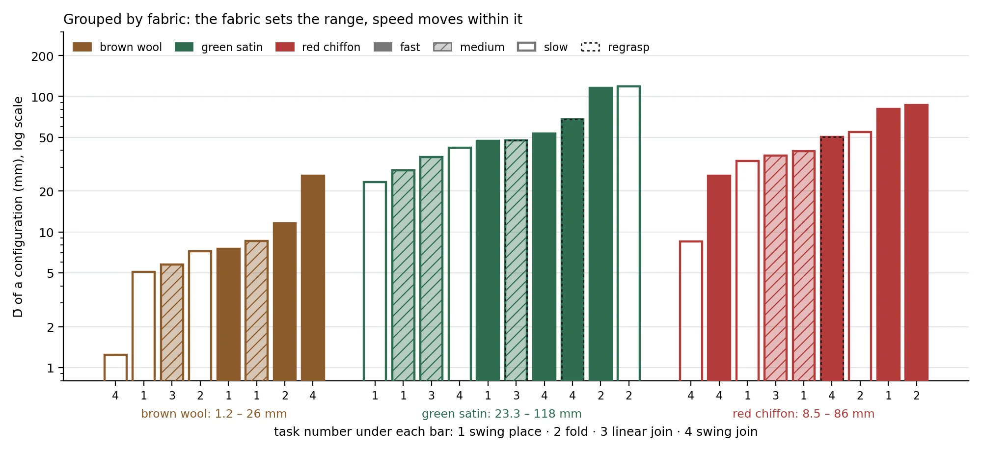
The variability changes dramatically, being the cloth type the dominant factor. If we group the 24 no-regrasp configurations by task or by speed and measure how much of the spread of log10 D̄c lies between the groups, the cloth explains 61 %, the task 10 % and the execution speed only 6 %. The brown cloth, the heaviest and highest-friction fabric, is, as expected, the most repeatable in every task except the fast swing join, where it reaches the same variability as the red cloth; the two light cloths scatter three to ten times more.
Regarding the speed contrast ΓD, the only value below 1 is the dynamic fold with the green satin (ΓD = 0.97), where the slower motion gets slightly more dispersion. For the rest of the tasks ΓD > 1, meaning higher velocity increases variability. The maximum value of ΓD corresponds to the brown wool in the swing join, with ΓD = 21, because this task is very repeatable at slow speed (only 1.2 mm of variability) but with the faster motion the variability increases very fast (to 25.9 mm). Regrasping the cloth before each rollout raises the floor variability to 12–27 mm instead of 2–4 mm, but the outcome still exceeds it by 2.6–4.2×, and compared to the same task without regrasp, regrasping does not significantly affect variability.
We show the variability amount for all tasks and their configurations with the whisker boxes of all the pair distances Dc(i,j) in all rollouts per configuration. The variability is orders of magnitude different depending on the task; that is why the y-axis is on a logarithmic scale.
Ten rollouts, one after another
The video shows one configuration, the terminal photograph of each rollout in turn and the cloth outlines stacked on one photograph. Here the same can be seen for every configuration. Where fewer than ten rollouts have a terminal mask the caption says how many are shown. D̄ is the configuration's value from the paper.
D̄ 115.2 mm · 10 rollouts
Captions of this scene in the video (fold, green satin, fast)
Ten terminal photographs, their outlines stacked: the cloth outcome varies
How D̄ is measured
In the video, D̄ is built on one configuration in thirteen seconds. Here we build it on one configuration of each task: the outcome markers of the ten rollouts, one pair of rollouts marker by marker, then every pair, and the same statistic on a grasped corner, which gives the floor ε.
D̄ 80.8 mm · ε 0.06 mm · 45 pairs of 10 rollouts
Captions of this scene in the video (swing place, red chiffon, fast)
Top view of the table: the free edge M01–M05 of each replay after landing, and the grasped corners M11, M15
Two replays: the distance marker by marker where both saw the marker, then the mean
Every pair of replays: 45 distances, one per cell · D̄ is their mean
On a grasped corner ε = 0.06 mm · D̄ / ε > 1000×: the cloth scatters, the robot does not
Through the motion
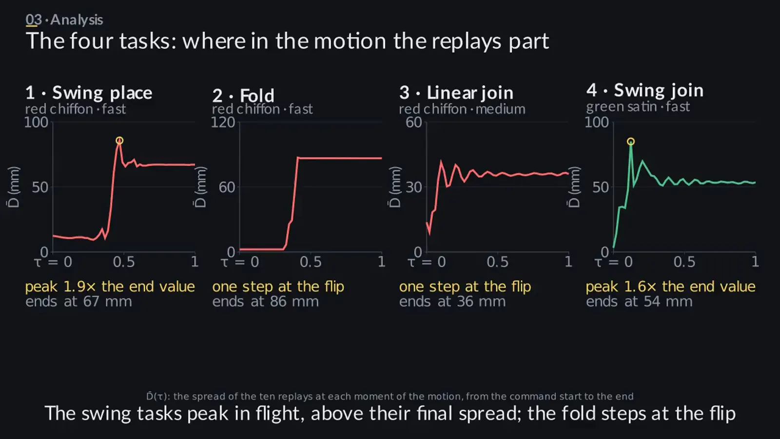
D̄(τ) is D̄ evaluated at each instant of the motion, from the command start to the settled end. One rollout is played with the markers of the other nine at the same instant, and D̄(τ) is drawn as the motion advances. All 27 configurations can be selected.
D̄ at the end 67 mm · peak 86 mm in flight, 1.3× the end value
Captions of this scene in the video (swing place, red chiffon, fast)
D̄(τ): the spread of the ten replays at each moment of the motion, from the command start to the end
The swing tasks peak in flight, above their final spread; the fold steps at the flip
One configuration per task, showing where in the motion the rollouts diverge. The two swing tasks peak in flight above their final value, and the fold steps at the flip.
All 27 configurations
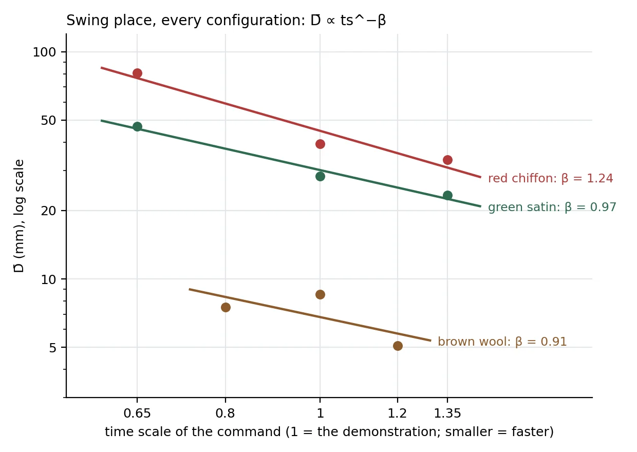
The video sorts the 27 configurations by D̄, groups them by cloth and fits the scaling of D̄ with speed for the swing place. The clip is followed by the same three views as figures.
Captions of this scene in the video
27 configurations sorted: two orders of magnitude
Grouped by fabric: the cloth type is the dominant factor
D̄ ∝ ts^−β: higher velocity increases the variability
The 27 configurations sorted by D̄c on a logarithmic scale, with the task number under each bar. The color is the cloth and the fill the speed; a dashed outline marks a regrasp configuration. * the lowest, 1.2 mm (brown wool, swing join, slow); ** the highest, 118 mm (green satin, fold, slow).The same bars grouped by cloth. The cloth sets the range and the speed moves within it.
The figure below shows how D̄c scales with the execution speed in the swing place. Each point is one configuration, D̄c against the time scale ts of the command, with one color per cloth and both axes logarithmic. ts = 1 is the recorded speed, 0.65 is 1.5 times faster and 1.35 is slower. On these axes the three points of a cloth line up, and a straight line on logarithmic axes is a power law, D̄c ∝ ts−β. The exponent β is the slope of that line. An execution k times faster multiplies D̄c by kβ, so with β = 1 twice as fast gives twice the spread. The fitted exponents are 0.91 for the brown wool, 0.97 for the green satin and 1.24 for the red chiffon, so the variability grows about in proportion to speed, and fastest for the lightest cloth. β carries the same information as the speed contrast ΓD of the paper, since ΓD = (ts,max / ts,min)β, and with three speeds the fit also uses the middle one.
D̄c of the swing place against the time scale ts on logarithmic axes, with one fitted line per cloth whose slope is its β.
Analysis of the variability per task
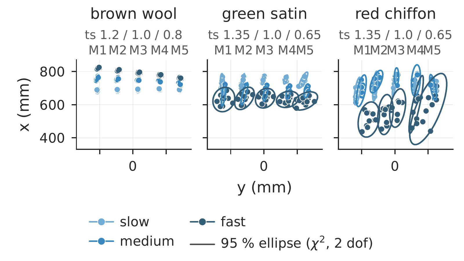
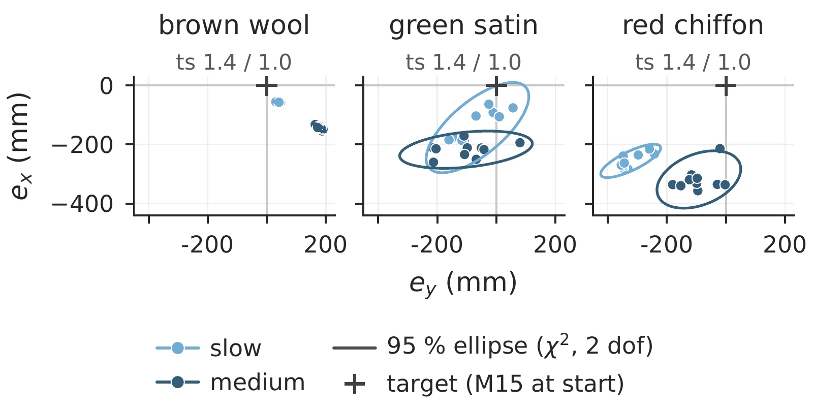
Swing place (task 1). Each dot in the figure is the resting point of one bottom-edge marker, m1 to m5, in one rollout; the darker the blue, the higher the execution speed. For the thick cloth the resting poses are less than a centimeter apart (5–9 mm) at every speed, while the two light cloths scatter 23–47 mm (green satin) and 33–81 mm (red chiffon), three to eleven times more, and their spread grows with speed while the heavy cloth's hardly does. The lighter and the more elastic the fabric, the more it disperses and the more speed matters. Every configuration exceeds its floor variability (εc ≤ 2.1 mm) by 14–1250×.
At slower speeds the variability is mainly in the direction of motion (X axis); for light cloths at high speed it also becomes very noticeable in the Y axis, indicating more complex aerodynamic effects.
Resting poses of the markers of the bottom edge for the swing place task (Task 1). It shows increasing variability for lighter cloths as well as with higher speeds.
Dynamic fold (task 2). We show the end location of the marker that swings to fold (m5) and its target, the position of m15; what we care about is not task success but how repeatable the folding motion is. The free corner lands away from its target in every configuration, by 7 to 41 cm. Clearly the best behaved is the thick fabric, with a dispersion of 7–12 mm against 55–118 mm for the light ones, whose flap sometimes crumples or folds instead of landing flat. Slowing the speed by 40 % does not significantly affect the result, and the floor variability is below 1 mm, 39–800 times less than at the free corner. These results indicate that this task is highly sensitive to cloth properties, and an optimized policy that reaches the target is unlikely to generalize across cloth types.
Resting poses of the free marker m5, with respect to the target pose for the task of dynamic folding (task 2). Variability of the lighter cloths are significantly bigger than for the thick brown cloth.
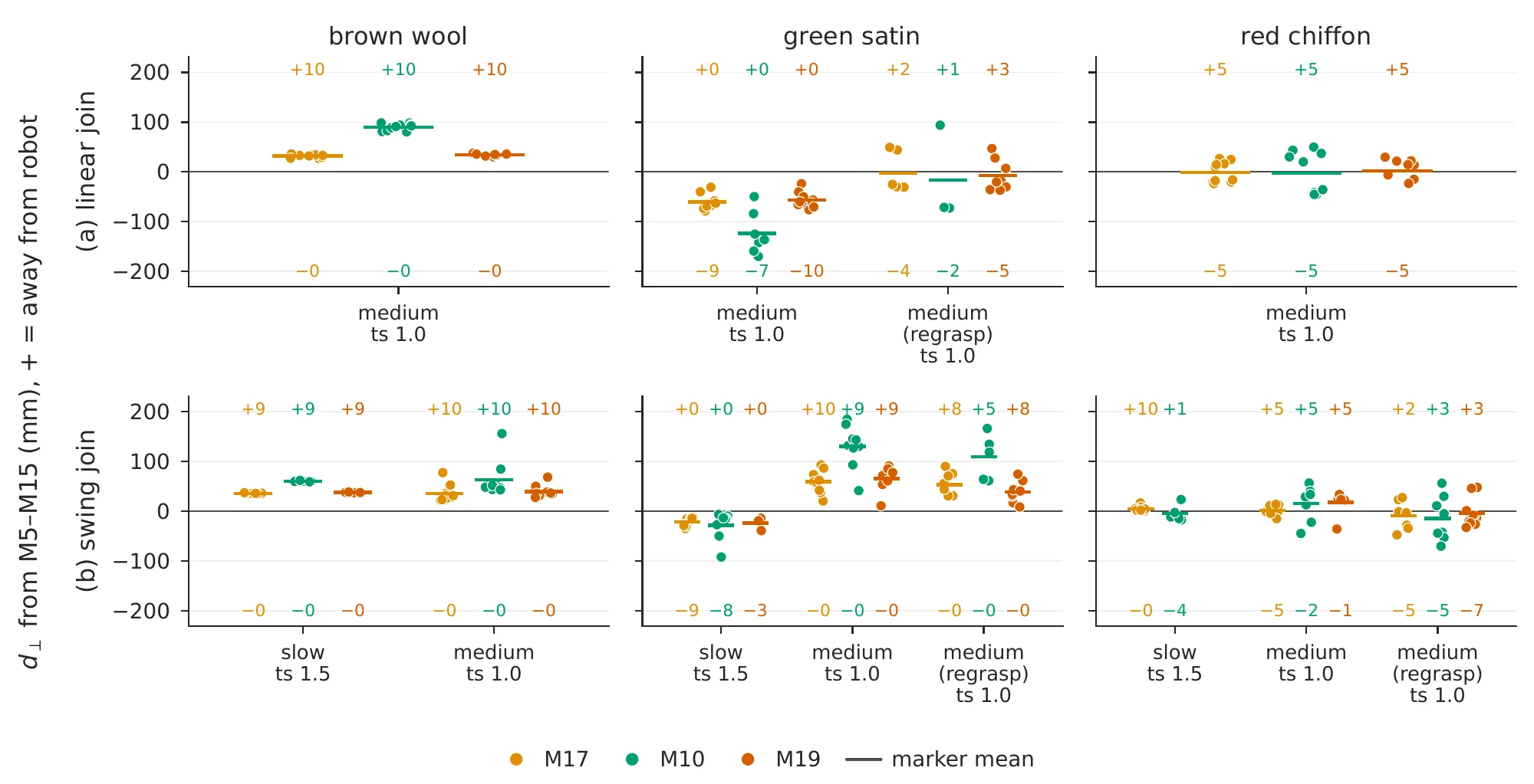
Linear and swing inward gripper motion (tasks 3 and 4). During the inward motion the grippers compress the top edge, which buckles out of the line m5–m15 with a magnitude d⊥; the figure shows d⊥ for each rollout, on top for the linear motion and at the bottom with the swing. For the stiff wool fabric the task is quite repeatable, and even without the swing the cloth was already buckling always to the same side with similar magnitude. The swing introduces more variability in the magnitude of d⊥, which may be positive to achieve a fold in the air but is less repeatable. For the green satin, at the same speed (ts = 1) the swing clearly forces the buckling towards the same side, also with regrasping, but at the slower speed the dynamics are not enough to ensure the direction. Finally, for the very soft red chiffon the swing does not seem to influence the outcome at all, at any speed. Looking at the videos, it is clear that for the swing to have the intended effect the grippers should come much closer before the swing finishes; otherwise, the cloth is soft enough to slide back to the other side in between the grippers. Even for humans, the swing motion with such a soft cloth is challenging.
For tasks 3 and 4, this graphic shows the amount of buckling (distance to line m5–m15 held by the grippers) described in the paper for the visible top cloth edge markers. The numbers at the top and bottom count the buckling side, using the paper.
Simulators
We replay every rollout of tasks 1 to 4 without regrasp in four cloth simulators, Clothilde, the PhysX cloth of Isaac Lab, the PBD cloth of Genesis and the VBD cloth of Newton, each calibrated per cloth with one set of material parameters for all four tasks. On eight held-out rollouts per cloth, two per task at the medium speed, the marker error is 37–48 mm for Clothilde, 70–78 mm for Isaac Lab, 82–90 mm for Genesis and 79–94 mm for Newton. The simulated markers are written back in the motion-capture file format, so the twin dataset runs through the same analysis code as the real one.
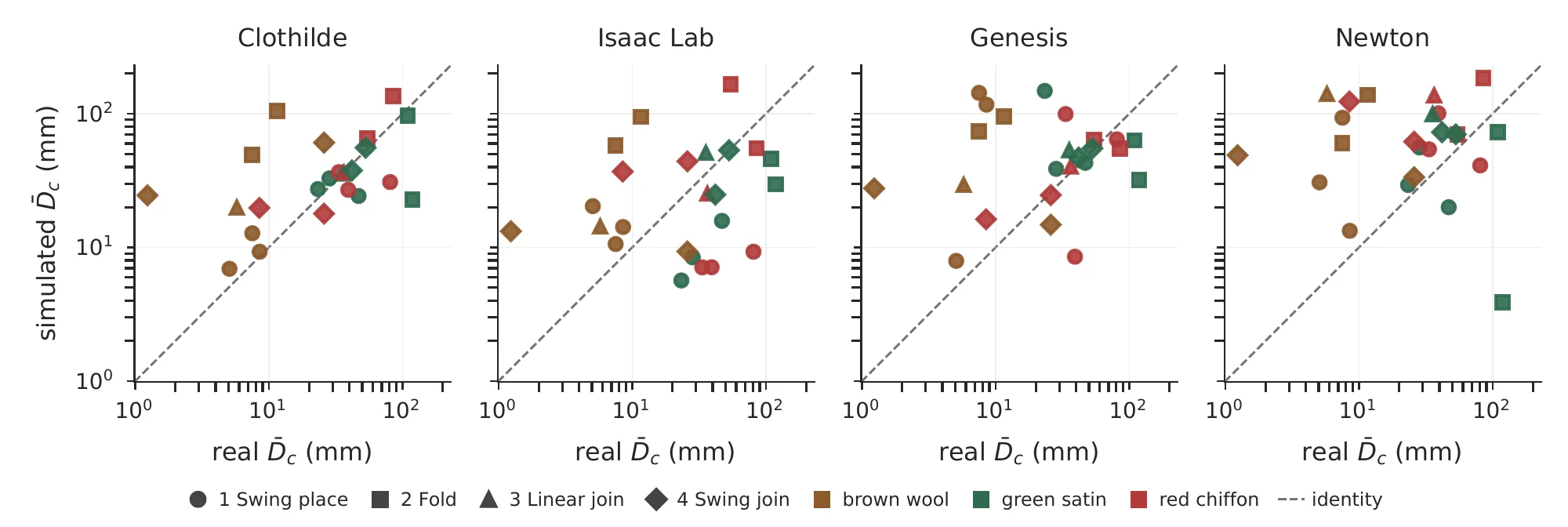
The figure plots the simulated dispersion of every calibrated engine against the real one; for a perfect simulation all dots would sit on the diagonal, sorted by the amount of variability. Note that even for deterministic simulators like Clothilde and Genesis, each rollout produces a different simulation, since each replay uses the measured start pose and gripper motion of its real rollout.
No engine reproduces the real variability. Clothilde and Genesis get the most points on the diagonal, particularly with the green satin and the red cloth, while the brown one is challenging for all simulators except Clothilde on the swing task. If we project the points on the X axis we get the ordering by amount of variability in the real cloth, and projecting on the Y axis gives the order in simulation. The order is not well preserved in any simulator, with Clothilde being slightly better thanks to the swing to place task. The same cloth under-disperses one task and over-disperses another, so in the simulators the dispersion is not related to the cloth properties.
Isaac Lab and Newton are not deterministic, so identical inputs do not replay identically. This noise is often as large as the real variability, but it is large where the real variability is small and vice versa, so the engine noise is not a replacement for the real variability.
Comparison of the variability amount in each simulator compared to the OptiTrack ground truth. Points closer to the diagonal correspond to more accurate simulations. None of the simulators captures the real variability.
Four simulators on one rollout
The four calibrated simulators replay one rollout of the configuration next to its video. Then, for each simulator, the resting positions of the ten simulated rollouts are shown against the ten real ones, with the ratio ρ = D̄sim / D̄real. All 24 no-regrasp configurations can be selected.
D̄ real 28 mm · Clothilde ρ 1.16 · Isaac Lab ρ 0.30 · Genesis ρ 1.36 · Newton ρ 1.97
Captions of this scene in the video (swing place, green satin, medium)
The calibrated engines replaying one real rollout
Real (white) vs simulated (color): where the ten landings fall · ρ = D̄ sim / D̄ real, 1 = the real spread
One rollout, full size
The rollout of the clip above in one simulator at a time and at full size. The simulated cloth is drawn in the simulator's color over the real markers, the arms are posed from the joint logs, and the stereo video plays inset in sync, all at real speed. The window runs from just before the cloth starts moving until it has settled. D̄ real and D̄ sim are the configuration's values from the simulator analysis and ρ their ratio.
D̄ real 28 mm · D̄ sim 33 mm · ρ 1.16
Measuring the dispersion without markers
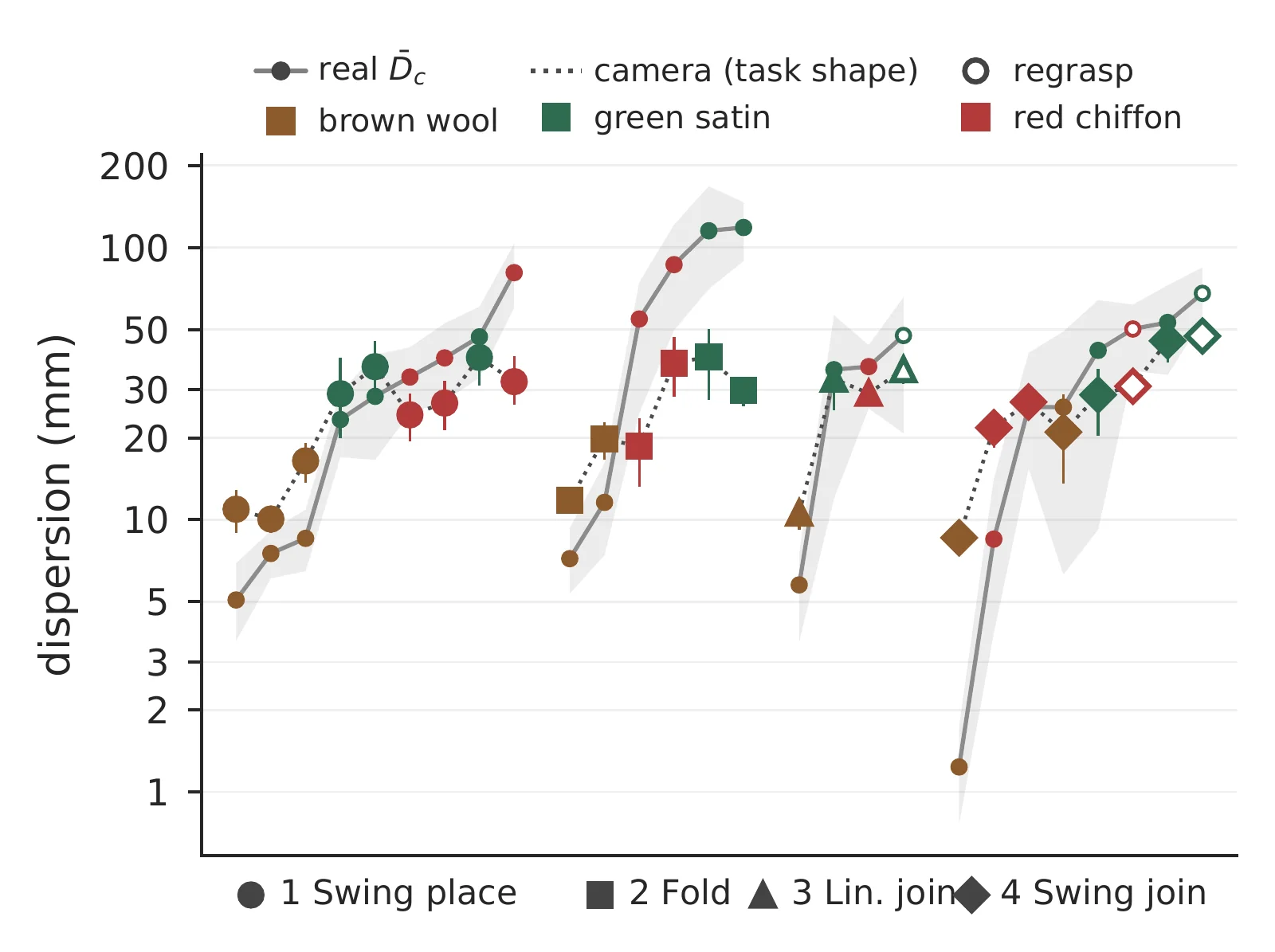
Motion capture is the most time-consuming part of the data collection, and most deployed policies use RGB(D) cameras, so we investigate how much of the same analysis we can perform without markers, using the stereo camera that recorded all our experiments. Each terminal state image is segmented with SAM 2, followed by 3-D extraction with FoundationStereo and described by DINOv3 patches; each patch takes the role of a virtual marker, and the mean distance between matched patches replaces the marker distance in D̄c.
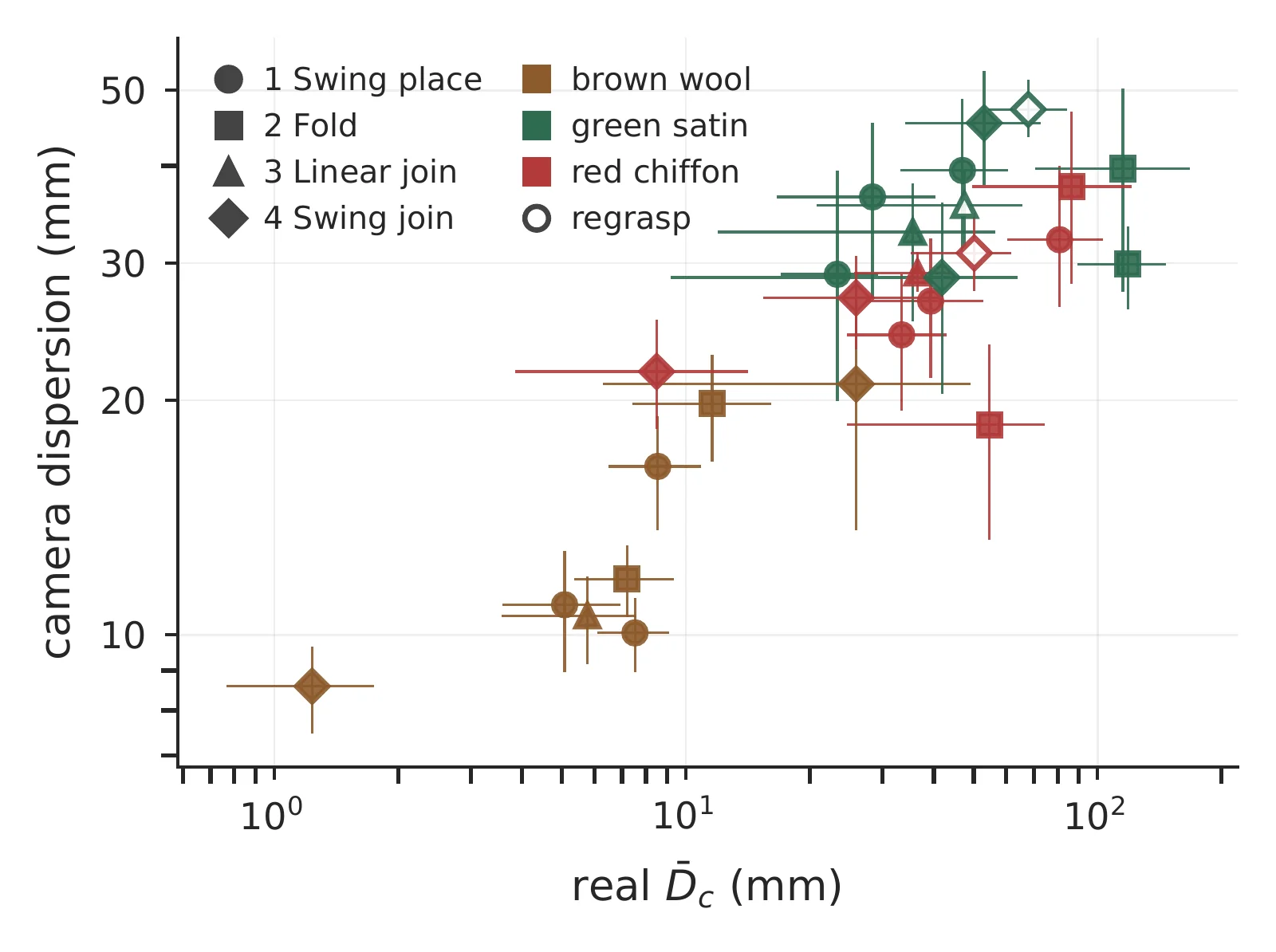
The figure shows the real variability of each task sorted in ascending order and the corresponding variability using vision. The general trend in the ordering is preserved, but variability is often overestimated or underestimated. In addition, perception struggles most in the dynamic fold task, where the free corner lands on the cloth, and as they have the same color the contrast is lost, leading to a big under-estimation of variability. The stereo camera with off-the-shelf models supports a qualitative comparison of cloths, speeds and tasks, but not a measurement of the dispersion itself with the precision provided by OptiTrack.
Variability using OptiTrack vs. using the markerless vision estimation. Although the trends are similar, vision does not capture the same variability values, nor the ordering.
Additional analysis
The analyses the paper defers to this page, computed as the paper defines them.
Every configuration: D̄c, the floor εc, their ratio and the speed contrast ΓD
The values behind the paper's results, one row per configuration: D̄c on the task's outcome markers, the floor εc on the grasped corners of the same rollouts, their ratio, and ΓD per cloth (D̄c at the fastest time scale over D̄c at the slowest), as defined in the paper. εc is given where at least three rollouts keep the grasped marker tracked to the end; the green satin fold has no such floor.
The floor εc of the paper is measured on the cloth corners held by the grippers, so it includes how the corner sits in the fingers, and it is an upper bound on the repeatability of the robot itself. The two additional columns report the same statistic on the markers of the grippers and on the logged tool pose, between 0.03 and 0.4 mm. With those floors, every no-regrasp configuration exceeds its floor by at least 5× and 9× respectively, and the regrasp configurations by more than 180×.
Task
Cloth
ts
Speed
Rollouts
D̄c (mm)
εc (mm)
D̄c / εc
ε on the gripper markers (mm)
ε on the logged tool pose (mm)
ΓD
1 Swing place
brown wool
0.8
fast
10
7.5
0.14
52
0.16
0.11
1.48
1 Swing place
brown wool
1
medium
10
8.5
0.62
14
0.04
0.04
1 Swing place
brown wool
1.2
slow
10
5.1
0.24
21
0.05
0.03
1 Swing place
green satin
0.65
fast
10
47.0
2.1
22
0.07
0.04
2.01
1 Swing place
green satin
1
medium
10
28.4
0.04
636
0.05
0.04
1 Swing place
green satin
1.35
slow
10
23.3
0.16
143
0.05
0.04
1 Swing place
red chiffon
0.65
fast
10
80.8
0.06
1252
0.07
0.06
2.42
1 Swing place
red chiffon
1
medium
10
39.3
0.06
614
0.08
0.06
1 Swing place
red chiffon
1.35
slow
10
33.4
0.73
46
0.06
0.03
2 Fold
brown wool
1
medium
10
11.6
0.23
49
0.09
0.08
1.61
2 Fold
brown wool
1.4
slow
10
7.2
0.18
39
0.18
0.09
2 Fold
green satin
1
medium
10
115.2
—
—
0.13
0.11
0.97
2 Fold
green satin
1.4
slow
10
118.4
—
—
0.09
0.06
2 Fold
red chiffon
1
medium
10
86.5
0.74
117
0.12
0.05
1.58
2 Fold
red chiffon
1.4
slow
10
54.6
0.07
800
0.15
0.07
3 Linear join
brown wool
1
medium
10
5.8
0.79
7.3
0.39
0.18
3 Linear join
green satin
1
medium
10
35.6
4.2
8.5
0.18
0.10
3 Linear join
green satin
1
medium (regrasp) (regrasp)
10
47.5
13.4
3.5
0.21
0.14
3 Linear join
red chiffon
1
medium
10
36.5
4.0
9.1
0.23
0.11
4 Swing join
brown wool
1
medium
10
25.9
0.53
49
0.24
0.11
20.96
4 Swing join
brown wool
1.5
slow
9
1.2
0.51
2.4
0.24
0.13
4 Swing join
green satin
1
medium
10
53.0
1.9
28
0.25
0.24
1.27
4 Swing join
green satin
1.5
slow
10
41.9
0.38
111
0.20
0.18
4 Swing join
green satin
1
medium (regrasp) (regrasp)
10
67.9
26.5
2.6
0.31
0.26
4 Swing join
red chiffon
1
medium
10
25.9
2.3
11
0.23
0.21
3.05
4 Swing join
red chiffon
1.5
slow
10
8.5
0.79
11
0.17
0.13
4 Swing join
red chiffon
1
medium (regrasp) (regrasp)
10
50.2
11.9
4.2
0.28
0.15
All markers of the joins (tasks 3 and 4)
The paper reports the top edge M17, M10, M19 for these two tasks and defers the resting positions of all markers to this page. Below, D̄c over every marker seen in both rollouts of a pair beside the top-edge value of the paper, and the terminal 3-D cloud of all 19 markers per configuration.
Task
Cloth
ts
Regrasp
D̄ top edge (mm)
D̄ all markers (mm)
markers per pair
3 Linear join
brown wool
1
no
5.8
3.0
18
3 Linear join
green satin
1
no
35.6
18.4
11
3 Linear join
green satin
1
yes
47.5
33.4
13
3 Linear join
red chiffon
1
no
36.5
30.4
16
4 Swing join
brown wool
1
no
25.9
19.2
19
4 Swing join
brown wool
1.5
no
1.2
4.0
19
4 Swing join
green satin
1
no
53.0
37.3
14
4 Swing join
green satin
1.5
no
41.9
16.8
14
4 Swing join
green satin
1
yes
67.9
45.8
14
4 Swing join
red chiffon
1
no
25.9
26.3
15
4 Swing join
red chiffon
1.5
no
8.5
16.0
14
4 Swing join
red chiffon
1
yes
50.2
29.8
14
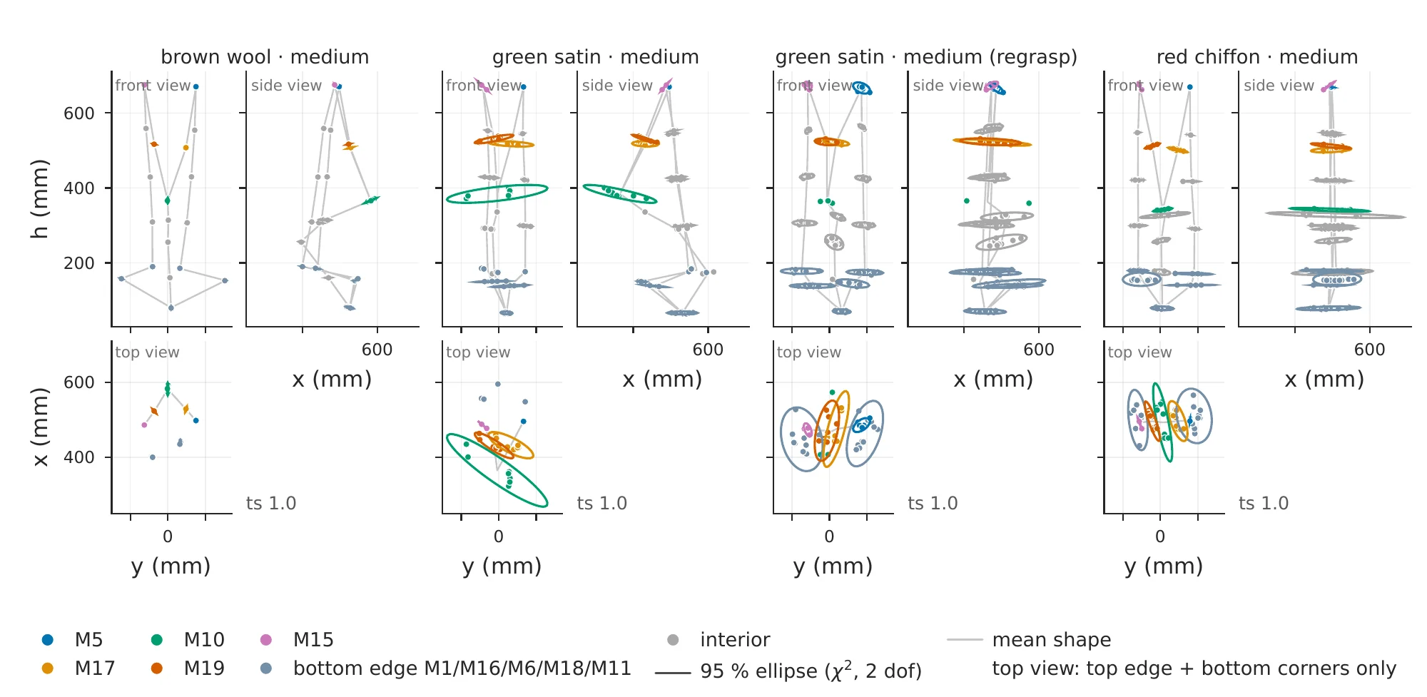
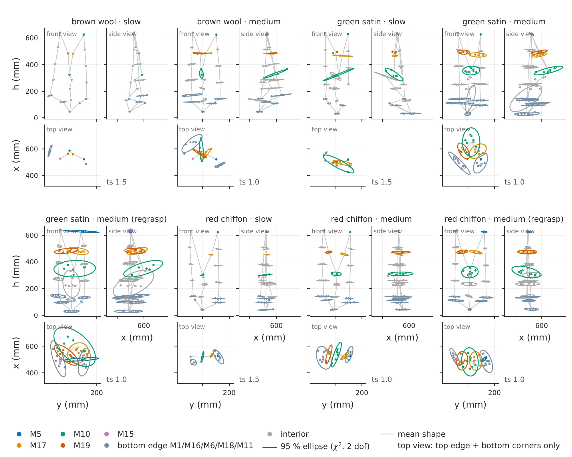
Linear join. The terminal position of all markers in three views, one dot per rollout, a 95 % ellipse per marker with at least five valid rollouts, the top edge and bottom corners highlighted, and the mean shape as a wireframe.Swing join, the same views for its eight configurations.The values of the simulator figure
The numbers plotted in the paper's simulator figure: the real D̄c of every no-regrasp configuration and the D̄c of its twins in the four engines (mm), then per engine and task the geometric mean of the ratio D̄sim / D̄real over the configurations (1 = the real spread), its range, and the Spearman rank correlation between the simulated and the real ordering of the configurations. The real D̄c is computed over the rollouts that have a twin. In three fold configurations one of the ten rollouts has none, so their value differs slightly from the per-configuration table above.
Task
Cloth
ts
rollouts compared
real D̄c (mm)
Clothilde
Isaac Lab
Genesis
Newton
1 Swing place
brown wool
0.8
10
7.5
12.8
10.6
143.4
93.4
1 Swing place
brown wool
1
10
8.5
9.3
14.2
117.0
13.3
1 Swing place
brown wool
1.2
10
5.1
6.9
20.4
7.9
30.7
1 Swing place
green satin
0.65
10
47.0
24.3
15.8
43.0
20.0
1 Swing place
green satin
1
10
28.4
32.9
8.4
38.7
56.0
1 Swing place
green satin
1.35
10
23.3
27.3
5.7
148.3
29.3
1 Swing place
red chiffon
0.65
10
80.8
30.9
9.3
64.4
41.1
1 Swing place
red chiffon
1
10
39.3
27.0
7.1
8.5
100.8
1 Swing place
red chiffon
1.35
10
33.4
36.6
7.1
99.5
54.2
2 Fold
brown wool
1
10
11.6
105.4
94.9
95.8
138.7
2 Fold
brown wool
1.4
9
7.5
49.2
57.9
74.0
60.3
2 Fold
green satin
1
9
109.3
96.8
45.9
63.3
73.0
2 Fold
green satin
1.4
10
118.4
22.8
29.7
32.0
3.9
2 Fold
red chiffon
1
9
85.2
135.4
55.2
54.7
184.6
2 Fold
red chiffon
1.4
10
54.6
65.2
165.6
63.7
70.3
3 Linear join
brown wool
1
10
5.8
19.9
14.4
29.4
140.9
3 Linear join
green satin
1
10
35.6
35.8
51.1
53.5
99.5
3 Linear join
red chiffon
1
10
36.5
36.3
25.3
40.3
137.5
4 Swing join
brown wool
1
10
25.9
60.8
9.3
14.8
33.6
4 Swing join
brown wool
1.5
9
1.2
24.5
13.2
27.7
49.0
4 Swing join
green satin
1
10
53.0
55.8
53.4
55.1
70.2
4 Swing join
green satin
1.5
10
41.9
37.7
24.8
47.1
72.8
4 Swing join
red chiffon
1
10
25.9
17.9
44.1
24.6
61.8
4 Swing join
red chiffon
1.5
10
8.5
19.8
37.0
16.2
123.6
Task
Engine
Configurations
geometric mean of D̄sim / D̄real
range
Spearman rank correlation
1 Swing place
Clothilde
9
0.93
0.38 – 1.7
+0.60
1 Swing place
Isaac Lab
9
0.46
0.11 – 4.0
-0.28
1 Swing place
Genesis
9
2.28
0.22 – 19.1
-0.15
1 Swing place
Newton
9
1.86
0.43 – 12.4
+0.08
2 Fold
Clothilde
6
1.64
0.19 – 9.1
-0.14
2 Fold
Isaac Lab
6
1.53
0.25 – 8.2
-0.77
2 Fold
Genesis
6
1.46
0.27 – 9.9
-0.89
2 Fold
Newton
6
1.34
0.03 – 12.0
-0.14
3 Linear join
Clothilde
3
1.51
0.99 – 3.5
+1.00
3 Linear join
Isaac Lab
3
1.35
0.69 – 2.5
+0.50
3 Linear join
Genesis
3
2.04
1.10 – 5.1
+0.50
3 Linear join
Newton
3
6.36
2.80 – 24.4
-0.50
4 Swing join
Clothilde
6
2.03
0.69 – 19.8
+0.60
4 Swing join
Isaac Lab
6
1.60
0.36 – 10.7
+0.37
4 Swing join
Genesis
6
1.73
0.57 – 22.4
+0.49
4 Swing join
Newton
6
4.00
1.29 – 39.6
+0.14
Over all 24 no-regrasp configurations, as in the video: the median miss is the factor by which half of an engine's configurations miss the real spread (exp of the median |ln D̄sim / D̄real|), the count of configurations within a factor of two of it, and the Spearman rank correlation with the real order of the configurations (1 would keep the real order).
Engine
median miss
within 2× of the real spread
rank correlation with the real order
Clothilde
1.45×
16 of 24
0.49
Genesis
1.74×
14 of 24
0.11
Newton
2.37×
10 of 24
0.01
Isaac Lab
3.00×
8 of 24
0.21
The camera's estimate per task, without markers
Per task, the agreement between the camera's estimate and the markers over the configurations: the Spearman rank correlation between the two orderings, the share of pairs of configurations of the same cloth that the camera puts in the markers' order, the ratio of the camera's dispersion to the markers' D̄c, and the median distance between a matched patch and the marker it stands for, at the grasped corners, the free edge and the free corners.
Task
Configurations
Spearman rank correlation with the markers
pairs of configurations of the same cloth in the markers' order
D̄ camera / D̄ markers
matched-patch error at grasped / edge / free markers (mm)
1 Swing place
9
0.77
89 %
0.89
14 / — / 7
2 Fold
6
0.77
67 %
—
— / — / —
3 Linear join
4
0.80
100 %
2.36
26 / 45 / 72
4 Swing join
8
0.93
100 %
2.25
22 / 23 / 71
Camera dispersion against the real D̄ of every configuration, both on logarithmic axes; hollow markers are the regrasp configurations.
Dataset
One episode per rollout, named <task>_eNN. Every stream is stamped on one clock and the metadata file carries the motion start and end index of each stream, so markers, frames and robot samples line up at any instant.
Stream
Files
Content
per episode
Motion capture
opti_<episode>.csv
OptiTrack Motive export (format 1.23), 100 Hz, world frame with x away from the robots and z up: the 19 cloth markers, the two end-effector rigid bodies (position and quaternion) and the four ArUco reference markers on the table. Marker labels were supervised manually.
≈ 1 MB
Robot logs
<episode>_robot_left.csv, _robot_right.csv
1 kHz: timestamp (s), the seven joint positions, TCP position and quaternion in the arm's base frame.
≈ 3 MB each
Stereo video
<episode>_zed.mkv, _zed_timestamps.npz
ZED 2i at 30 Hz, side-by-side stereo 2 × 1280 × 720, lossless FFV1, with per-frame timestamps.
Cloth, time scale, regrasp flag, grasp preset, controller, and the motion start and end index in every stream; a replay-accuracy plot of desired versus achieved joint trajectories.
—
Simulator twins
one folder per engine, opti_<episode>.csv
The simulated markers of every no-regrasp rollout, written in the same motion-capture format so the same analysis runs on real and simulated data.
≈ 0.8 GB per engine
Totals: motion capture 0.4 GB, robot logs 2 GB, stereo video 62 GB (mkv) plus 161 GB of ZED recordings, simulator twins ≈ 3.5 GB for the four engines.
One rollout per task, the stereo frame beside its 3-D reconstruction from the logs on one clock.
Download
Sample data. One complete swing-place episode (red chiffon, medium speed): core files (13 MB: motion capture, robot logs, metadata, terminal stills, the four simulator twins, the engine-agnostic replay inputs, the calibrated parameters of the four engines, the camera calibration and a README of the file schema), the lossless stereo video (270 MB) and a viewing copy of it (8 MB, H.264).*
* For double-blind review, some metadata (recording dates, camera identifiers) is removed and a small rectangle over a wall poster is masked in the video frames; the measurements are untouched.
Full release. The 269 rollouts with their stereo streams and simulator twins, under a persistent identifier, with a loader.
License. CC BY 4.0.
Reading one episode
import pandas as pd, yaml
# OptiTrack export: skip the format line; header rows = asset name, Rotation/Position, axis
opti = pd.read_csv("opti_swing_place_e00.csv", skiprows=1, header=[1, 3, 4])
m05  = opti["Cloth:Marker_05"]["Position"][["X", "Y", "Z"]]            # one cloth marker, meters, world frame
robot = pd.read_csv("swing_place_e00_robot_left.csv", index_col=0)   # 1 kHz joints + TCP
meta  = yaml.safe_load(open("swing_place_e00_metadata.yaml"))         # cloth_type, time_scale, sync indices